Neutron CW Powder Data - Yttrium Iron/Aluminium Garnet
In this tutorial you will refine the structure of yttrium iron/aluminum garnet using constant wavelength neutron data. The structure is cubic with four different atomic sites two of which are occupied by both iron and aluminum. The data was taken on the D1a powder diffractometer at the ILL, Grenoble, France using 1.909Å wavelength neutrons.
If you have not done so already, start GSAS-II.
Step 1: read in the data file
1. Use the Import/Powder Data/from GSAS file menu item to read the data file into GSAS-II. This read option is set to read any of the powder data formats (except neutron TOF time map files) defined for GSAS (angles in centidegrees). Other submenu items will read the cif format or the xye format (angles in degrees) used by Topas, etc. Change the file directory to CWNeutron/data to find the file; you will need to change the file type to All files (*.*) to find the desired file.
2. Select the garnet.raw data file in the first dialog and press Open. There will be a Dialog box asking Is this the file you want? Press Yes button to proceed.
3. Select the inst_d1a.prm instrument parameter file in the second dialog and press Open.
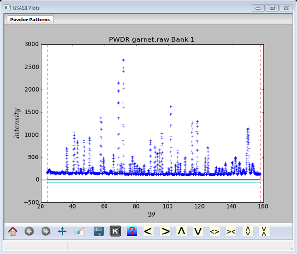
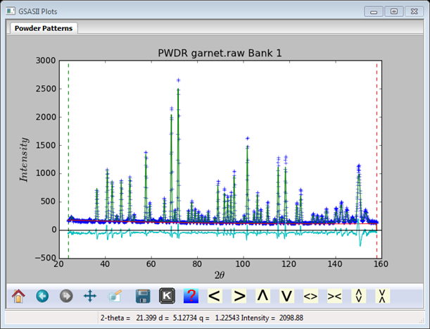
At this point the left side of GSAS-II Data Window (the GSAS-II data tree) will have several entries and the plot window will show the powder pattern
Step 2: Create the phase
Use the Data/Add phase menu item to begin creation of the new phase for this garnet; enter a phase name in the dialog box, we assume ‘garnet’. The default phase information will immediately be displayed.
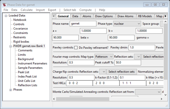
The General tab is visible; scroll bars can be used or you can resize the window to see the rest of the data. The Phase type is correctly set to “nuclear”; other options can be used for other structural problems (e.g. magnetic or faulted). Press the space group box (shows “P 1”), and enter the space group ‘I a 3 d’ (spaces between axial fields are required in GSAS-II) in the popup window and press OK, the space group information window will appear

Press OK to exit. The General tab display will change (principally changes in lattice parameter display). Enter the lattice parameter for garnet (a=12.19) in the appropriate field and press Enter. The display will change again to show the cell volume.
Click on the Data
tab and select Edit Phase/Add powder histograms
in the menu for this window. A Use data
window will appear with only one choice PWDR garnet.raw: BANK 1. Select it and press OK. The Data
tab will change
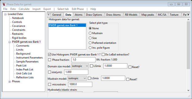
This window is the home of parameters that are both phase and data set dependent. These include phase fraction, crystallite size, mustrain & preferred orientation.
Step 3. Insert the atoms
Click on the Atoms tab; this is where you will insert the atoms for the garnet structure. The 6 sets of atom coordinates are:
|
TYPE |
X |
Y |
Z |
|
Y |
0.12500 |
0. 00000 |
0. 25000 |
|
FE |
0.00000 |
0.00000 |
0.00000 |
|
AL |
0.00000 |
0.00000 |
0.00000 |
|
AL |
0.37500 |
0.00000 |
0.25000 |
|
FE |
0.37500 |
0.00000 |
0.25000 |
|
O |
-0.03000 |
0.05000 |
0.15000 |
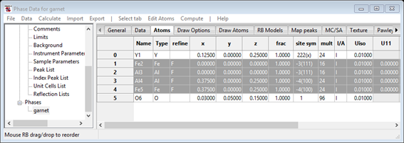
To begin use the Edit/Append atom in the menu on the Atoms tab 6 times to create the default set of atom places in the table; the table will look like
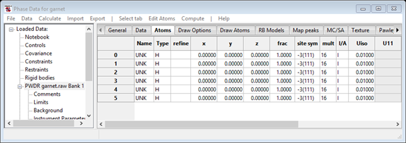
Then for each atom to be inserted, double click on the “H” in the Type column; a Periodic Table will appear

Each element has a small pull down selection for the possible valences (usually choose the “zero” one). Select “Y”, the Table will vanish and the Name and Type for that atom will change. Then enter the values for x, y and z; you can use Tab to move to the next one. You may use fractions for the atom coordinates (e.g. 1/4, 3/8). Do this for each atom in the Atoms table. NB: be careful about the signs for the O-atom positions. You can leave both frac and Uiso at the default values. Your result should look like

You can now do your first Rietveld refinement on this problem. To do this, do Calculate/Refine in the left side of the menu; a file
dialog will ask you for a name for this project; you can change the directory
if you wish. We assume the name “YAG”;
the current project will be saved as YAG.gpx
and the first backup file (YAG.bak0.gpx)
will also be created and then the Rietveld refinement will be performed. By
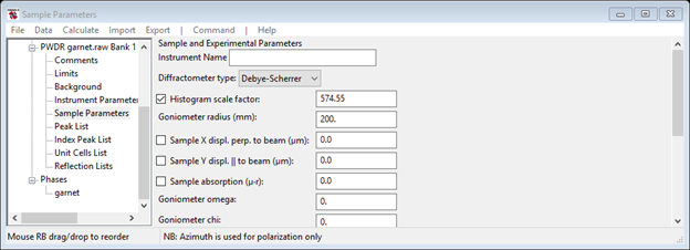
default, only the histogram scale factor (found under Sample
Parameters for PWDR garnet.raw: BANK1 in the GSAS-II
data tree) and 3 background coefficients are refined. The resulting
powder pattern
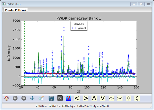
shows a pretty poor fit (Rwp ~39%) and details can be found in the YAG.lst file. What appears to be in error includes some structural features (I’d first suspect site fractions for the Fe/Al sites) and something about the peak positions (may be lattice parameter). We can introduce all these parameters now.
1. Go to Phases/garnet and check Refine unit cell in the General tab.
2. Next go to Constraints in the main part of the GSAS-II data tree (near the top). You will see an empty window with 3 tabs; Phase is the one you want. Select Edit Constr./Add equivalence from the menu. You will see the following new window
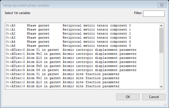
select 0::AUiso:1 for Fe2… and press OK; a new window will appear
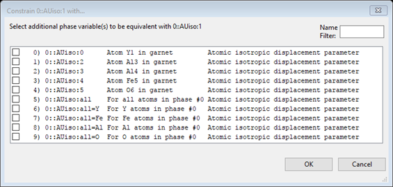
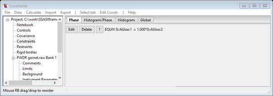
select 0::AUiso:2 for Al3 and press OK. That will form the first equivalence you need between the Fe and Al atoms that occupy the atom site at 0,0,0 in the cell. This shows up in the Constraints window.
Now do the same for the atoms 0::AUiso:3 for Al4 and 0::AUiso:4 for Fe5 to make that pair of atoms have the same Uiso.
3. Next select Edit Constr./Add constraint equation. A now familiar window will appear; select 0::Afrac:1 for Fe2 and press OK. Again you will see the same second window; select 0::Afrac:2 for Al3 and press OK. Do the same thing for 0::Afrac:3 for Al4 – you may have to scroll down the list to see this – and 0::Afrac:4 for Fe5. When done the Constraints window should look like

This process set the equivalences/constraints for the two Fe/Al sites in the garnet so that refinement of frac and Uiso will succeed. GSAS-II constraints will correct the site fractions and Uiso values so that they conform to the constraints as written. You need not be concerned about their starting values beforehand. Also note the way each parameter was named; the general form is p:h:name:num where p is a phase number, h is a histogram number, name is the parameter name and num is an optional number (e.g. an atom number).
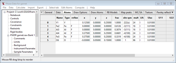
4. Go to the Phases/garnet item in the GSAS-II data tree and select the Atoms tab. Note the frac values are unchanged from what you originally entered. Don’t worry, they will be corrected in the next refinement. We now have to set the refinement of frac for the Fe/Al sites. There are many ways to do this, we will show you one method now. Select row 1 for Fe(2) and then holding the Ctrl key down select rows 2-4; they will appear all blue or gray. Next select Edit Atoms/On selected atoms…/Refine selected; a new window will appear
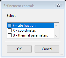
For now select F – site fraction. You could select all three, GSAS-II would refine frac & Uiso but not the coordinates as they are fixed as special positions in this case. The Atom window will have an F in the refine column each of these atoms.
You are now ready for your second Rietveld refinement; select Calculate/Refine from the left side of the menu bar. There is now a much better fit with Rwp ~12% and a powder pattern that looks like (select PWDR garnet.raw from the GSAS-II data tree to see it)

There appears to be some differences in peak intensities and an interesting offset at the low end of the pattern. Let us add the remaining atom parameters (Uiso for each and the O(xyz) parameters. Go to Phases/garnet and select the Atoms tab.
Notice that the frac values for the Fe/Al atoms now conform to the constraints. For each atom in turn, double click on the refine box. A pull down list will appear, select U for the Y atom, FU for Fe/Al atoms and XU for the O atom. Your list should look like
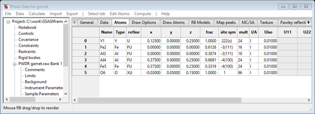
when done. Now you can do your third Rietveld refinement; select Calculate/Refine. The resulting fit is
with Rwp ~10%. There is still an apparent peak offset at the ends of the pattern and perhaps some misfit of the peak widths.
The latter are determined by the U, V & W parameters found in the PWDR garnet.raw: BANK1/Instrument Parameters window. Go there and select their Refine? flags (these are the checkboxes next to GSAS-II parameters). Next go to Sample Parameters.
Notice that the Histogram scale factor is already being refined. Now you will want to refine both Sample X displacement and Sample Y displacement. The values will be in mm if the Goniometer radius is correct; enter 650 for that value. Now you can do another Rietveld refinement; the fit
is nearly perfect! Rwp = 5.18%. You can look at the YAG.lst output file for all the parameters and their respective esds. I’ve pasted some of my results in below for you to compare.
Refinement
results:
---------------------------------------------------------------------------------------------------------------------------------------
Number of function calls: 7 Number of observations: 2677
Number of parameters: 20
Refinement time = 3.448s,
0.862s/cycle, for 4 cycles
wR = 5.18%, chi**2 = 10072.9, reduced chi**2 = 3.79
----------------------------------------------------------------------------------------------------------------------------------
Variables
generated by constraints
name
: 0::AUiso:1 0::AUiso:3 0::A0 ::constr0 ::constr1
value : 0.0035 -0.0004 0.0067 -0.1083
-0.2843
sig :
0.0006 0.0007 0.0000 0.0127 0.0104
Phases:
Result for phase: garnet
Reciprocal metric tensor:
names : A11 A22 A33 A12 A13 A23
values:
0.006738782 0.006738782 0.006738782 0.000000000 0.000000000 0.000000000
esds : 0.000000268
New unit cell:
names : a
b c alpha beta gamma Volume
values:
12.181739 12.181739 12.181739
90.0000 90.0000 90.0000
1807.706
esds : 0.000242
0.036
Atoms:
name
x y z
frac Uiso U11 U22
U33 U12 U13
U23
---------------------------------------------------------------------------------------------------------------------------------------
Y(1) Y:
values:
0.12500 0.00000 0.25000
1.000 0.00442
sig : 0.00035
Fe(2) Fe:
values:
0.00000 0.00000 0.00000
0.577 0.00347
sig : 0.009 0.00059
Al(3) Al:
values:
0.00000 0.00000 0.00000
0.423 0.00347
sig : 0.009 0.00059
Al(4) Al:
values:
0.37500 0.00000 0.25000
0.701-0.00041
sig : 0.007 0.00074
Fe(5) Fe:
values:
0.37500 0.00000 0.25000
0.299-0.00041
sig : 0.007 0.00074
O(6) O:
values:
-0.02942 0.05390 0.15059
1.000 0.00472
sig :
0.00006 0.00006 0.00007 0.00027
Phase: garnet in
histogram: PWDR garnet.raw
Bank 1
----------------------------------------------------------------------------------------------------------------------------------
Final refinement RF, RF^2 = 2.27%, 3.70% on 89
reflections
Bragg intensity sum = 2.74e+05
Histogram:
PWDR garnet.raw Bank 1 histogram Id: 0
---------------------------------------------------------------------------------------------------------------------------------------
PWDR histogram weight factor = 1.000
Final refinement wR
= 5.18% on 2677 observations in this histogram
Other residuals: R = 4.22%, Rb = 3.40%, wRb = 3.55% wRmin = 2.67%
Instrument type: Debye-Scherrer
Sample Parameters:
names : Scale Absorption DisplaceX DisplaceY
values:
612.9203 0.0000
1242.4926 -2837.8867
sig :
3.4719
53.7322 117.5487
Instrument Parameters:
names : Lam
Polariz.
SH/L U V W X
value : 1.909000
0.000000 0.002000 258.609371 -645.406449 572.149553
0.000000
sig :
4.221864 10.112266 5.820126
Instrument Parameters:
names : Y Zero
value : 0.000000
-0.129218
sig : 0.005984
Background function: chebyschev
value : 121.3
-27.19 27.04
sig :
0.2834 0.537 0.9925
Background sums: empirical 2.41e+04, Debye 0,
peaks 0, Total 2.41e+04
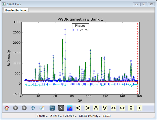
A useful display to examine is given by selecting Covariance in the GSAS-II data tree
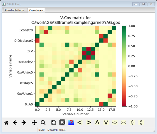
This is a graphical rendering of the variance-covariance matrix from the last refinement. This matrix is symmetric about the diagonal; moving your cursor about it will display parameter names, values and esds on the diagonal and the covariance between a pair of parameters off the diagonal. Intense red or green indicates high covariance (green for + and red for -) and yellow is for close to zero covariance. High covariances naturally occur for profile coefficients and for background parameters. You can change the color scheme, the default is RdYlGn. If during the course of one of your refinements you see white bands in this display: that is the signature of some singularities in your refinement. The offending parameter(s) should not be refined independently; perhaps a constraint/equivalence is needed.